
Señales en MATLAB
Objetivo
Generar gráficas de funciones básicas de señales con Matlab
Fundamento teórico
Desarrollo
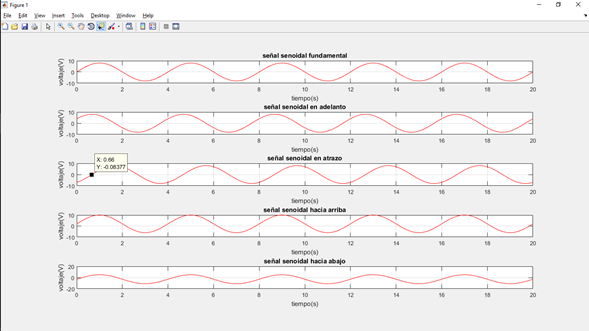
- Onda senoidal
-Codigo para generar la onda senoidal con Matlab
- %Generación de señales sinoidales
- clc
- clear all
- close all
- %Tiempo
- t=0:0.01:20;
- %Amplitud
- A=8;
- %Periodo(s)
- T=4;
- %Frecuencia (Hz)
- f=1/T;
- %Frecuencia angular (rad/s)
- w=2*pi*f;
- %Señal sinoidal fundamental
- v1=A*sin(w*t);
- %Señal sinoidal en adelanto
- v2=A*sin(w*t+pi/6);
- %Señal sinoidal en atraso
- v3=A*sin(w*t-pi/3);
- %Señal sinoidal desfazada hacia arriba
- v4=A*sin(w*t)+2;
- %Señal sinoidal desfasada hacia abajo
- v5=A*sin(w*t)-3;
- %Gráfica de las señales
- subplot 511
- plot(t,v1,'r')
- xlabel('tiempo(s)')
- ylabel('voltaje(V)')
- title('señal senoidal fundamental')
- grid on
- subplot 512
- plot(t,v2,'r')
- xlabel('tiempo(s)')
- ylabel('voltaje(v)')
- title('señal senoidal en adelanto')
- grid on
- subplot 513
- plot(t,v3,'r')
- xlabel('tiempo(s)')
- ylabel('volaje(V)')
- title('señal senoidal en atrazo')
- grid on
- subplot 514
- plot(t,v4,'r')
- xlabel('tiempo(s)')
- ylabel('volaje(V)')
- title('señal senoidal hacia arriba')
- grid on
- subplot 515
- plot(t,v5,'r')
- xlabel('tiempo(s)')
- ylabel('volaje(V)')
- title('señal senoidal hacia abajo')
- grid on
-Gráfica de las funciones senoidales
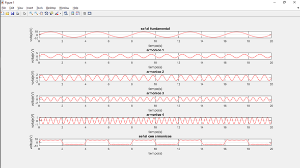
- Señal con armónicos
-Codigo para generación de señales con armónicos con Matlab
- %Generación de señales con armónicos
- clc
- clear all
- close all
- %Tiempo
- t=0:0.01:20;
- %Amplitud
- A=8;
- %Periodo(s)
- T=4;
- %Frecuencia (Hz)
- f=1/T;
- %Frecuencia angular (rad/s)
- w=2*pi*f;
- %Señal sinoidal fundamental
- v1=A*sin(w*t);
- %Señal armónico 1
- v2=(A/3)*sin(3*w*t);
- %Señal armónico 2
- v3=(A/5*sin(5*w*t);
- %Señal armónico 3
- v4=(A/7)*sin(7*w*t);
- %Señal armónico 4
- v5=(A/9)*sin(9*w*t);
- %Señal total
- v6=v1+v2+v3+v4+v5;
- %Gráfica de las señales
- subplot 611
- plot(t,v1,'r')
- xlabel('tiempo(s)')
- ylabel('voltaje(V)')
- title('señal fundamental')
- grid on
- subplot 612
- plot(t,v2,'r')
- xlabel('tiempo(s)')
- ylabel('voltaje(v)')
- title('armónico 1')
- grid on
- subplot 613
- plot(t,v3,'r')
- xlabel('tiempo(s)')
- ylabel('volaje(V)')
- title('armónico 2')
- grid on
- subplot 614
- plot(t,v4,'r')
- xlabel('tiempo(s)')
- ylabel('volaje(V)')
- title('armónico 3')
- grid on
- subplot 615
- plot(t,v5,'r')
- xlabel('tiempo(s)')
- ylabel('volaje(V)')
- title('armónico 4')
- grid on
- subplot 616
- plot(t,v6,'r')
- xlabel('tiempo(s)')
- ylabel('voltaje(V)')
- title('señal con armonicos')
- grid on
-Gráfica de las señales con armónicos
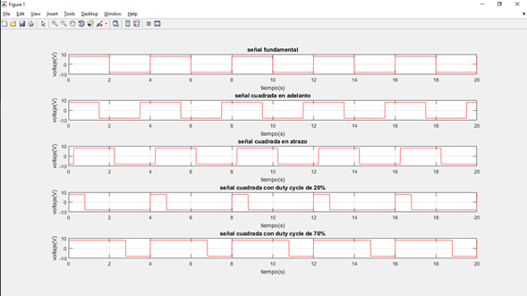
- Onda cuadrada
-Código para generación de una señal cuadrada:
- %Generación de onda cuadrada
- clc
- clear all
- close all
- %Tiempo
- t=0:0.01:20;
- %Amplitud
- A=8;
- %Periodo(s)
- T=4;
- %Frecuencia (Hz)
- f=1/T;
- %Frecuencia angular (rad/s)
- w=2*pi*f;
- %Señal cuadrada fundamental
- v1=A*square(w*t);
- %Señal cuadrada en adelanto
- v2=A*square(w*t+pi/4);
- %Señal cuadrada en atraso
- v3=A*square(w*t-pi/8);
- %Señal cuadrada con duty cycle de 20%
- v4=A*square(w*t,20); %el 20 esta en porcentaje
- %Señal cuadrada con duty cycle de 70%
- v5=A*square(w*t,70);
- %Gráfica de las señales
- subplot 511
- plot(t,v1,'r')
- xlabel('tiempo(s)')
- ylabel('voltaje(V)')
- title('señal fundamental')
- grid on
- subplot 512
- plot(t,v2,'r')
- xlabel('tiempo(s)')
- ylabel('voltaje(v)')
- title('señal cuadrada en adelanto')
- grid on
- subplot 513
- plot(t,v3,'r')
- xlabel('tiempo(s)')
- ylabel('volaje(V)')
- title('señal cuadrada en atrazo')
- grid on
- subplot 514
- plot(t,v4,'r')
- xlabel('tiempo(s)')
- ylabel('volaje(V)')
- title('señal cuadrada con duty cycle de 20%')
- grid on
- subplot 515
- plot(t,v5,'r')
- xlabel('tiempo(s)')
- ylabel('volaje(V)')
- title('señal cuadrada con duty cycle de 70%')
- grid on
-Gráfica de las señales cuadradas
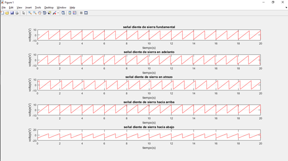
- Señal diente de sierra (Sawtooth)
-Codigo para generación de la señal diente de sierra con Matlab
- %Generación de señales diente de sierra
- clc
- clear all
- close all
- %Tiempo
- t=0:0.01:20;
- %Amplitud
- A=8;
- %Periodo(s)
- T=1;
- %Frecuencia (Hz)
- f=1/T;
- %Frecuencia angular (rad/s)
- w=2*pi*f;
- %Señal diente de sierra fundamental
- v1=A*sawtooth(w*t);
- %Señal diente de sierra en adelanto
- v2=A*sawtooth(w*t+pi/6);
- %Señal diente de sierra en atraso
- v3=A*sawtooth(w*t-pi/3);
- %Señal diente de sierra desfazada hacia arriba
- v4=A*sawtooth(w*t)+2;
- %Señal diente de sierra desfasada hacia abajo
- v5=A*sawtooth(w*t)-3;
- %Gráfica de las señales
- subplot 511
- plot(t,v1,'r')
- xlabel('tiempo(s)')
- ylabel('voltaje(V)')
- title('señal diente de sierra fundamental')
- grid on
- subplot 512
- plot(t,v2,'r')
- xlabel('tiempo(s)')
- ylabel('voltaje(v)')
- title('señal diente de sierra en adelanto')
- grid on
- subplot 513
- plot(t,v3,'r')
- xlabel('tiempo(s)')
- ylabel('volaje(V)')
- title('señal diente de sierra en atrazo')
- grid on
- subplot 514
- plot(t,v4,'r')
- xlabel('tiempo(s)')
- ylabel('volaje(V)')
- title('señal diente de sierra hacia arriba')
- grid on
- subplot 515
- plot(t,v5,'r')
- xlabel('tiempo(s)')
- ylabel('volaje(V)')
- title('señal diente de sierra hacia abajo')
- grid on
-Gráfica de las señales diente de sierra (Sawtooth)
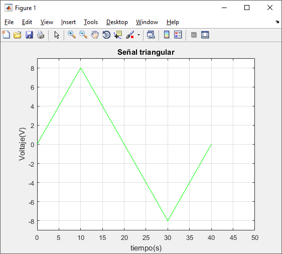
- señal triangular
-Codigo para generar la señal triangular con Matlab
- %Generación de señales triangular
- clc
- clear all
- close all
- %Tiempo
- t=0:0.01:40;
- %Amplitud
- A=8;
- %Periodo(s)
- T=40;
- %voltaje
- v1=(t>= & t<=T/4).*(4*A*t/T);
- v2=(t>T/4 & t<=3*T/4).*(-4*A*t/T+2*A);
- v3=(t>3*T/4 & t<=T).*(4*A*t/T - 4*A);
- v=v1+v2+v3;
- plot(t,v,'g')
- grid on
- xlabel('tiempo(s)')
- ylabel('voltaje(V)')
- title('señal triangular')
- axis ([0 50 -9 9])
-Gráfica de la señal triangular
Conclusiones
Desarrollo
- Onda senoidal
-Codigo para generar la onda senoidal con Matlab
- %Generación de señales sinoidales
- clc
- clear all
- close all
- %Tiempo
- t=0:0.01:20;
- %Amplitud
- A=8;
- %Periodo(s)
- T=4;
- %Frecuencia (Hz)
- f=1/T;
- %Frecuencia angular (rad/s)
- w=2*pi*f;
- %Señal sinoidal fundamental
- v1=A*sin(w*t);
- %Señal sinoidal en adelanto
- v2=A*sin(w*t+pi/6);
- %Señal sinoidal en atraso
- v3=A*sin(w*t-pi/3);
- %Señal sinoidal desfazada hacia arriba
- v4=A*sin(w*t)+2;
- %Señal sinoidal desfasada hacia abajo
- v5=A*sin(w*t)-3;
- %Gráfica de las señales
- subplot 511
- plot(t,v1,'r')
- xlabel('tiempo(s)')
- ylabel('voltaje(V)')
- title('señal senoidal fundamental')
- grid on
- subplot 512
- plot(t,v2,'r')
- xlabel('tiempo(s)')
- ylabel('voltaje(v)')
- title('señal senoidal en adelanto')
- grid on
- subplot 513
- plot(t,v3,'r')
- xlabel('tiempo(s)')
- ylabel('volaje(V)')
- title('señal senoidal en atrazo')
- grid on
- subplot 514
- plot(t,v4,'r')
- xlabel('tiempo(s)')
- ylabel('volaje(V)')
- title('señal senoidal hacia arriba')
- grid on
- subplot 515
- plot(t,v5,'r')
- xlabel('tiempo(s)')
- ylabel('volaje(V)')
- title('señal senoidal hacia abajo')
- grid on
-Gráfica de las funciones senoidales
- Señal con armónicos
-Codigo para generación de señales con armónicos con Matlab
- %Generación de señales con armónicos
- clc
- clear all
- close all
- %Tiempo
- t=0:0.01:20;
- %Amplitud
- A=8;
- %Periodo(s)
- T=4;
- %Frecuencia (Hz)
- f=1/T;
- %Frecuencia angular (rad/s)
- w=2*pi*f;
- %Señal sinoidal fundamental
- v1=A*sin(w*t);
- %Señal armónico 1
- v2=(A/3)*sin(3*w*t);
- %Señal armónico 2
- v3=(A/5*sin(5*w*t);
- %Señal armónico 3
- v4=(A/7)*sin(7*w*t);
- %Señal armónico 4
- v5=(A/9)*sin(9*w*t);
- %Señal total
- v6=v1+v2+v3+v4+v5;
- %Gráfica de las señales
- subplot 611
- plot(t,v1,'r')
- xlabel('tiempo(s)')
- ylabel('voltaje(V)')
- title('señal fundamental')
- grid on
- subplot 612
- plot(t,v2,'r')
- xlabel('tiempo(s)')
- ylabel('voltaje(v)')
- title('armónico 1')
- grid on
- subplot 613
- plot(t,v3,'r')
- xlabel('tiempo(s)')
- ylabel('volaje(V)')
- title('armónico 2')
- grid on
- subplot 614
- plot(t,v4,'r')
- xlabel('tiempo(s)')
- ylabel('volaje(V)')
- title('armónico 3')
- grid on
- subplot 615
- plot(t,v5,'r')
- xlabel('tiempo(s)')
- ylabel('volaje(V)')
- title('armónico 4')
- grid on
- subplot 616
- plot(t,v6,'r')
- xlabel('tiempo(s)')
- ylabel('voltaje(V)')
- title('señal con armonicos')
- grid on
-Gráfica de las señales con armónicos
- Onda cuadrada
-Código para generación de una señal cuadrada:
- %Generación de onda cuadrada
- clc
- clear all
- close all
- %Tiempo
- t=0:0.01:20;
- %Amplitud
- A=8;
- %Periodo(s)
- T=4;
- %Frecuencia (Hz)
- f=1/T;
- %Frecuencia angular (rad/s)
- w=2*pi*f;
- %Señal cuadrada fundamental
- v1=A*square(w*t);
- %Señal cuadrada en adelanto
- v2=A*square(w*t+pi/4);
- %Señal cuadrada en atraso
- v3=A*square(w*t-pi/8);
- %Señal cuadrada con duty cycle de 20%
- v4=A*square(w*t,20); %el 20 esta en porcentaje
- %Señal cuadrada con duty cycle de 70%
- v5=A*square(w*t,70);
- %Gráfica de las señales
- subplot 511
- plot(t,v1,'r')
- xlabel('tiempo(s)')
- ylabel('voltaje(V)')
- title('señal fundamental')
- grid on
- subplot 512
- plot(t,v2,'r')
- xlabel('tiempo(s)')
- ylabel('voltaje(v)')
- title('señal cuadrada en adelanto')
- grid on
- subplot 513
- plot(t,v3,'r')
- xlabel('tiempo(s)')
- ylabel('volaje(V)')
- title('señal cuadrada en atrazo')
- grid on
- subplot 514
- plot(t,v4,'r')
- xlabel('tiempo(s)')
- ylabel('volaje(V)')
- title('señal cuadrada con duty cycle de 20%')
- grid on
- subplot 515
- plot(t,v5,'r')
- xlabel('tiempo(s)')
- ylabel('volaje(V)')
- title('señal cuadrada con duty cycle de 70%')
- grid on
-Gráfica de las señales cuadradas
- Señal diente de sierra (Sawtooth)
-Codigo para generación de la señal diente de sierra con Matlab
- %Generación de señales diente de sierra
- clc
- clear all
- close all
- %Tiempo
- t=0:0.01:20;
- %Amplitud
- A=8;
- %Periodo(s)
- T=1;
- %Frecuencia (Hz)
- f=1/T;
- %Frecuencia angular (rad/s)
- w=2*pi*f;
- %Señal diente de sierra fundamental
- v1=A*sawtooth(w*t);
- %Señal diente de sierra en adelanto
- v2=A*sawtooth(w*t+pi/6);
- %Señal diente de sierra en atraso
- v3=A*sawtooth(w*t-pi/3);
- %Señal diente de sierra desfazada hacia arriba
- v4=A*sawtooth(w*t)+2;
- %Señal diente de sierra desfasada hacia abajo
- v5=A*sawtooth(w*t)-3;
- %Gráfica de las señales
- subplot 511
- plot(t,v1,'r')
- xlabel('tiempo(s)')
- ylabel('voltaje(V)')
- title('señal diente de sierra fundamental')
- grid on
- subplot 512
- plot(t,v2,'r')
- xlabel('tiempo(s)')
- ylabel('voltaje(v)')
- title('señal diente de sierra en adelanto')
- grid on
- subplot 513
- plot(t,v3,'r')
- xlabel('tiempo(s)')
- ylabel('volaje(V)')
- title('señal diente de sierra en atrazo')
- grid on
- subplot 514
- plot(t,v4,'r')
- xlabel('tiempo(s)')
- ylabel('volaje(V)')
- title('señal diente de sierra hacia arriba')
- grid on
- subplot 515
- plot(t,v5,'r')
- xlabel('tiempo(s)')
- ylabel('volaje(V)')
- title('señal diente de sierra hacia abajo')
- grid on
-Gráfica de las señales diente de sierra (Sawtooth)
- señal triangular
-Codigo para generar la señal triangular con Matlab
- %Generación de señales triangular
- clc
- clear all
- close all
- %Tiempo
- t=0:0.01:40;
- %Amplitud
- A=8;
- %Periodo(s)
- T=40;
- %voltaje
- v1=(t>= & t<=T/4).*(4*A*t/T);
- v2=(t>T/4 & t<=3*T/4).*(-4*A*t/T+2*A);
- v3=(t>3*T/4 & t<=T).*(4*A*t/T - 4*A);
- v=v1+v2+v3;
- plot(t,v,'g')
- grid on
- xlabel('tiempo(s)')
- ylabel('voltaje(V)')
- title('señal triangular')
- axis ([0 50 -9 9])
-Gráfica de la señal triangular
Conclusiones
Por lo antes mostrado es visible que Matlab es un software que vuelve practico el cálculo y la muestra grafica de señales fundamentales en electrónica.